This animation is dedicated to my advisor Upmanu Lall, who’s been so supportive of all my many projects, including this one! Prabhat Barnwal and I have been studying the effects of Hurricane Sandy on the New York area through the lens of twitter emotions, ever since we propitiously began collecting tweets a week before the storm emerged (see the working paper).

The animation shows every geolocated tweet in between October 20 and November 5, across much of the Northeastern seaboard– about 2 million tweets in total.

Each tweet is colored based on our term-usage analysis of its emotional content. The hue reflects happiness, varying from green (happy) to red (sad), greyer colors reflect a lack of authority, and darker colors reflect a lack of engagement. The hurricane, as a red circle, jutters through the bottom-left of the screen the night of Oct. 29.

The first thing to notice is how much more tweeting activity there is near the hurricane and the election. Look at the difference between seconds 22 (midnight on Oct. 25) and 40 (midnight on Oct. 30).

The night of the hurricane, the tweets edge toward pastel as people get excited. The green glow near NYC that each night finishes with becomes brighter, but the next morning the whole region turns red as people survey the disaster.

My girlfriend uses a “Moka Express”-style stovetop Bialetti espresso-maker most mornings for her cappuccino. These devices are wonderful, reliable, and simple, but they have a nearly fatal flaw. A basin collects the espresso as it condenses, and for the five minutes before the steam brewing happens, there will be no indication of anything happening. Then espresso will start to quietly gurgle up, and if you don’t stop the process in the 20 seconds after it starts, the drink will be ruined.

I built a simple device to solve this problem. It has two wires that sit in the basin, and a loud buzzer that sounds as soon as coffee touches them.

How it works

Here is the circuit diagram for the coffee buzzer, designed to be powered by a 9V battery:

The core of the coffee buzzer is a simple voltage divider. Normally, when the device is not in coffee, the resistance through the air between the two leads on the left (labeled “LOAD”) is very high. As a result, the entire voltage from 9V battery is applied to that gap, so that the voltage across the 500 KΩ resistor is 0.

The IRF1104 is a simple MOSFET, which acts like a voltage-controlled switch. With no voltage across the resistor, the MOSFET is off, so the buzzer doesn’t sound.

To turn the MOSFET on, the voltage across the 500 KΩ resistor needs to be about 2 V. As a result, anything between the two LOAD leads with a resistance of less than about 2000 KΩ will cause the buzzer to turn on.

Coffee resistance seems to vary quite a bit, and the 137 KΩ shown here is on the low end. For this, you need a resistor of at least 40 KΩ. I suggest using something higher, so the detector will be more sensitive.

What you need

Tools

You will need wire-strippers, a multimeter (to check your circuit), and a soldering iron (to put everything together).

Parts

These wires will be the main detector of the coffee buzzer.

Here I use a 1500 KΩ resistor, so the buzzer will sound for resistances less than 5000 KΩ will be detected. Make sure that you use a resistor of more than 300 KΩ.

The MOSFET is a voltage controlled switch, and it’s what allows the buzzer to get plenty of current even though there’s a lot of resistance for current moving through the coffee.

You can get a 9V battery connector (top) and a buzzer (middle, rated for between 4 and 8 V) at RadioShack or from DigiKey. And, of course, the battery itself (not included).

Optional (but highly recommended!)

A simple switch (which may look very different from this one) is a great way to build an integrity tester into the device itself.

A breadboard will let you put the whole circuit together and test it before you solder it.

Wires like these make plugging everything into a breadboard easier.

I suggest taping up the whole device after you solder it, both for protection and to keep everything in one tight package.

How to make an Espresso Buzzer

Start by preparing the detector wires (the black and white wires above). Take at least 30 cm of wire, so the device can sit on the counter away from the flame. Use the wire stripper to strip one end of the wires for use in the circuit. You may want to strip the “detection” end, or not: if you leave the detector end unstripped, the buzzer won’t go off prematurely when if both wires touch the bottom of the basin, but you’ll have to wipe off the end of the wires to get them to stop buzzing once they have started.

Now connect all of the pieces on the breadboard. Here’s one arrangement:

If you aren’t sure how to use a breadboard or how to read a circuit diagram, you can still make the buzzer by skipping this step and soldering the wires together as specified below.

Once everything is connected on the breadboard, you should be able to test the coffee buzzer. If you use a switch, pressing it should make the buzzer sound. Then make a little experimental coffee, and dip the leads into the coffee to check that it works.

Next, solder it all together. As you can see in the circuit diagram, you want to solder together the following groups of wires:

• Ground: The black wire from the battery connector; one wire from the resistor; and the source lead on the MOSFET (furthest right).
• Power: The red wire from the battery connector; one wire from the buzzer; the (stripped) circuit end of one of the detector wires; and optionally one end of the switch.
• Gate: The (stripped) circuit end of the other detector wire; the other end of the resistor; the gate lead on the MOSFET (furthest left); and optionally the other end of the switch.
• Buzzer: The gate lead on the MOSFET (middle); and the remaining wire to the buzzer.

After you have soldered everything together, test it and then wrap tape around it all.

The results

That’s it! Now, to use it, place the detector leads at the bottom of the coffee basin. I suggest putting a bend into the wires a couple inches from the end, so they can sit easily in the basin. If you’ve stripped the ends, the buzzer may buzz when the leads touch the base, but if you just let them go at this point, one wire will sit slightly above the other and just millimeters away from the bottom for perfect detection.

As soon as the coffee reaches a level where both leads are submerged, the detector will start buzzing!

Enjoy!

R doesn’t have a built-in method for calculating heteroskedastically-robust and clustered standard errors. Since this is a common need for us, I’ve put together a little library to provide these functions.

Download the library.

The file contains three functions:

• get.coef.robust: Calculate heteroskedastically-robust standard errors
• get.coef.clust: Calculate clustered standard errors
• get.conf.clust: Calculate confidence intervals for clustered standard errors

The arguments for the functions are below, and then an example is at the end.

get.coef.robust(mod, var=c(), estimator=”HC”)
Calculate heteroskedastically-robust standard errors

mod: the result of a call to lm()
     e.g., lm(satell ~ width + factor(color))
var: a list of indexes to extract only certain coefficients (default: all)
     e.g., 1:2 [to drop FE from above]
estimator: an estimator type passed to vcovHC (default: White's estimator)
Returns an object of type coeftest, with estimate, std. err, t and p values

get.coef.clust(mod, cluster, var=c())
Calculate clustered standard errors

mod: the result of a call to lm()
     e.g., lm(satell ~ width + factor(color))
cluster: a cluster variable, with a length equal to the observation count
     e.g., color
var: a list of indexes to extract only certain coefficients (default: all)
     e.g., 1:2 [to drop FE from above]
Returns an object of type coeftest, with estimate, std. err, t and p values

get.conf.clust(mod, cluster, xx, alpha, var=c())
Calculate confidence intervals for clustered standard errors

mod: the result of a call to lm()
     e.g., lm(satell ~ width + factor(color))
cluster: a cluster variable, with a length equal to the observation count
     e.g., color
xx: new values for each of the variables (only needs to be as long as 'var')
     e.g., seq(0, 50, length.out=100)
alpha: the level of confidence, as an error rate
     e.g., .05 [for 95% confidence intervals]
var: a list of indexes to extract only certain coefficients (default: all)
     e.g., 1:2 [to drop FE from above]
Returns a data.frame of yhat, lo, and hi

Example in Stata and R

The following example compare the results from Stata and R for an example from section 3.3.2 of “An Introduction to Categorical Data Analysis” by Alan Agresti. The data describes 173 female horseshoe crabs, and the number of male “satellites” that live near them.

Download the data as a CSV file. The columns are the crabs color (2-5), spine condition (1-3), carapace width (cm), number of satellite crabs, and weight (kg).

The code below calculates a simple model with crab color fixed-effects, relating width (which is thought to be an explanatory variable) and number of satellites. The first model is a straight OLS regression; then we add robust errors, and finally crab color clustered errors.

The analysis in Stata.

First, let’s do the analysis in Stata, to make sure that we can reproduce it in R.

import delim data.csv

xi: reg satell width i.color
xi: reg satell width i.color, vce(hc2)
xi: reg satell width i.color, vce(cluster color)

Here are excerpts of the results.

The OLS model:

------------------------------------------------------------------------------
      satell |      Coef.   Std. Err.      t    P>|t|     [95% Conf. Interval]
-------------+----------------------------------------------------------------
       width |   .4633951   .1117381     4.15   0.000     .2428033    .6839868
       _cons |  -8.412887   3.133074    -2.69   0.008    -14.59816   -2.227618
------------------------------------------------------------------------------

The robust errors:

------------------------------------------------------------------------------
             |             Robust HC2
      satell |      Coef.   Std. Err.      t    P>|t|     [95% Conf. Interval]
-------------+----------------------------------------------------------------
       width |   .4633951   .1028225     4.51   0.000     .2604045    .6663856
       _cons |  -8.412887   2.939015    -2.86   0.005    -14.21505   -2.610726
------------------------------------------------------------------------------

Note that we’ve used HC2 robust errors, to provide a direct comparison with the R results.

The clustered errors.

------------------------------------------------------------------------------
             |               Robust
      satell |      Coef.   Std. Err.      t    P>|t|     [95% Conf. Interval]
-------------+----------------------------------------------------------------
       width |   .4633951   .0466564     9.93   0.002     .3149135    .6118767
       _cons |  -8.412887   1.258169    -6.69   0.007    -12.41694   -4.408833
------------------------------------------------------------------------------

The robust and clustered errors are a little tighter for this example.

The analysis in R.

Here’s the equivalent code in R.

source("tools_reg.R")
tbl <- read.csv("data.csv")

mod <- lm(satell ~ width + factor(color), data=tbl)

summary(mod)
get.coef.robust(mod, estimator="HC2")
get.coef.clust(mod, tbl$color)

And excerpts of the results. The OLS model:

               Estimate Std. Error t value Pr(>|t|)    
(Intercept)     -8.4129     3.1331  -2.685  0.00798 ** 
width            0.4634     0.1117   4.147 5.33e-05 ***

The coefficient estimates will be the same for all three models. Stata gives us -8.412887 + .4633951 w and R gives us -8.4129 + 0.4634 w. These are identical, but with different reporting precision, as are the standard errors.

The robust errors:

(Intercept)    -8.41289    2.93902 -2.8625  0.004739 ** 
width           0.46340    0.10282  4.5067 1.229e-05 ***

Again, we use HC2 robust errors. Stata provides 2.939015 and .1028225 for the errors, matching these exactly.

The clustered errors:

                Estimate Std. Error  t value  Pr(>|t|)    
(Intercept)    -8.412887   1.258169  -6.6866 3.235e-10 ***
width           0.463395   0.046656   9.9321 < 2.2e-16 ***

Stata gives the exact same values as R.

I’ve started a long project of identifying my top 500 articles and chapters– the papers that either had a great impact on me or that I keep returning to to illustrate a point. One of those is Jeremey Jackson et al. (2001), Historical overfishing and the recent collapse of coastal ecosystems.

The main argument– that overfishing precedes, predicts, and predisposes the present fragility of ecosystems to modern drivers like pollution– is less interesting than the case studies themselves: kelp forests, coral reefs, seagrass beds, oyster estuaries, and benthic communities. This before-after diagram drives the point home (I colored the changes):

The most depressing line is in the abstract:

Paleoecological, archaeological, and historical data show that time lags of decades to centuries occurred between the onset of overfishing and consequent changes in ecological communities, because unfished species of similar trophic level assumed the ecological roles of overfished species until they too were overfished or died of epidemic diseases related to overcrowding.

Maybe questions of social science never get truly resolved. The first year of my PhD, I remember John Mutter describing the question of creative destruction. Sometimes, the story goes, a disaster can lead to an unexpected silver lining. By destroying outdated infrastructure, or motiving people to work together, or driving a needed influx of aid, a disaster can eventually leave a community better off than beforehand. Mutter described it almost like a philosophical quandary. In the face of all the specifics of institutions, internal perceptions, and international relations, how will we ever know?

For years now, Solomon Hsiang has been producing insights from his LICRICE model, turning hurricanes into exogenous predictors. As these random shocks echo through societies, he’s been picking up everything that falls out. I got to listen to some of it when news reporters would call his office. His work with Jesse Anttila-Hughes turned up the true mortality threat of disasters, typically 10x the lives lost at the time of the event. Jesse dug further, finding how family assets changed, how meals were redistributed, and how young girls are often the most hurt, even those born after the disaster.

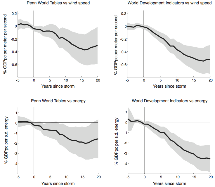
Last month, Sol and Amir Jina produced an NBER working paper that steps back from the individual lives affected. Their result is that a single storm produces losses that continue to accumulate for 20 years. People are not only continuing to feel the effects of a hurricane 20 years down the road, but they additional poverty they feel at 10 years is only half of the poverty that they’ll feel in another 10.

Of course, this is an average effect, and an average of 6415 different country results. But that means that for every country that experiences no long-term effect, one experiences twice the poverty.

So, is there creative destruction? It’s very, very unlikely. The most likely situation is “no recovery”: countries will never return to the trend that they were on prior to the event. Things are even more dire under climate change,

For a sense of scale, our estimates suggest that under the “Business as usual” scenario (with a 5% discount rate) the [present discounted value] of lost long-run growth is $855 billion for the United States (5.9% of current GDP), $299 billion for the Philippines (83.3% of current GDP), $1 trillion for South Korea (73% of current GDP), $1.4 trillion for China (12.6% of current GDP), and $4.5 trillion for Japan (101.5% of current GDP).

That’s what we should be willing to pay to avoid these costs. In comparison to the $9.7 trillion that just additional hurricanes are expected to cost, the $2 trillion that Nordhaus (2008) estimates for the cost of a climate policy seems trivial. That’s two big, seemingly unanswerable questions as settled as things get in social science.

Sometimes a diagram helps me find order in chaos, and sometimes it’s just a way to stroke my ego. I was recently trying to make sense of my graduate school classes, even as they’re becoming a less and less important share of my gradschool learning. So, I added to a diagram I’d made ten years ago for college.  In the end, I’m not sure which purpose it serves more.

The diagram is arrayed by discipline and year. The disciplines are arranged like a color wheel (and classes colored accordingly), from theoretical math, through progressively more applied sciences, through engineering and out the other end into applied humanities (like music), and finally back to theoretical philosophy. Arrows give a sense of thematic and prerequisite relationships.

Economics, a core of the Sustainable Development program, probably sits around the back-side of the spectrum, between philosophy and math. I squeezed it in on the left, more as a reflection of how I’ve approached it than what it tried to teach.

This is also missing everything I’ve learned from classes I’ve taught. I wish there were a place for Progressive Alternatives from two years ago, or Complexity Science from last year. I guess I need another diagram.

I’m running a pair of seminars to introduce people to python, for the purpose of extracting data from various online sources.  I still need to write up the content of the seminars, with plenty of examples at from trivial to intermediate.  But first, I wanted to post the diagram I did for myself, to think about how to organize all of this material: a diagram.

How do the elements of python connect to each other, how do they relate to elements on the web, and how do elements on the web related to each other?

Boxes are python elements and ovals are web elements. I aimed to cover everything in brown, touch on items in blue, and at-most mention items in grey.

Sol, Amir, and I have been slaving away over a report on the business-case for fighting climate change.  And it was released this morning!  The media outlets give a sense of the highlights:

Take a look!  Here’s the media report:
http://riskybusiness.org/report/overview/executive-summary

And the scientific report (what we actually helped write):
http://rhg.com/reports/climate-prospectus

I’m in a group studying Bayesian techniques for environmental research, under Upmanu Lall at the Earth Institute. We recently did a session on the packages available in R for modeling Bayesian Networks. Here’s the spreadsheet that came out of the meeting: