A month of nominal changes

I’ve been busy! In the last month, I have collected an appalling list of achievements which mean much to the world and very little to life as I live it.

First, I am a doctor, as of May 20. Not a real doctor, and Flame won’t let me wear a stethoscope anyway. But my program in sustainable development is officially over. Interestingly, this is nothing like job changes I have had before: I still work on the same projects and attend the same meetings with the same people. But in theory, I am now unemployed, and I will soon be a UC Berkeley employee with similarly slight impacts.

Second, I can now drive a car. Of course, I could before, and have been acceptably competent at it for the past six months. But the winter is a horrible time to take a road test, and New York City is a horrible place for one. My license was finally approved on Monday. I have yet to experience the joys or sorrows of driving alone, but I hear California is great for that.

I have also finished my Hepatitis A and B shot series and gotten a new Yellow Fever vaccination. I think I was already immune with the first shots, and only people who lose their international immunization card need a second Yellow Fever vaccine, but now I have paperwork for all three. And, twelve years out, I am not quite done with my student loans, but with $101.58 left, I might as well be.

Flame and I are now ensconced in a tiny apartment on the corner of Prospect Park, Brooklyn. Officially we have had the apartment for over a month, but we just changed residences last week. So, I suppose with all of the nominal changes, there are a few real ones too. It has been an exciting journey! But some time I will need at least a nominal vacation.

Google Scholar Alerts to RSS: A punctuated equilibrium

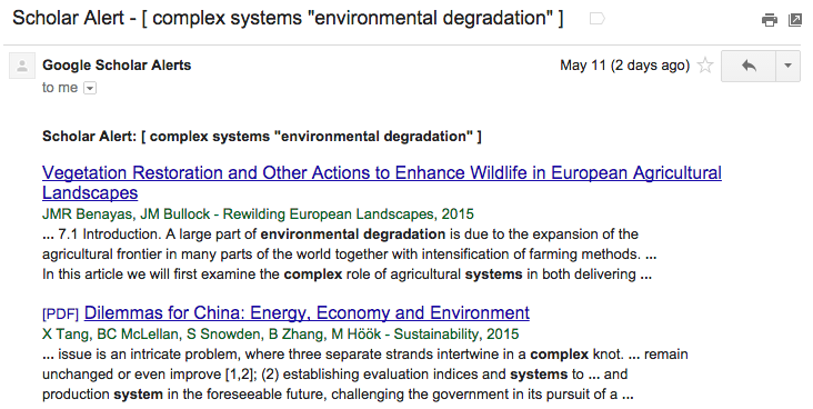
If you’re like me, you have a pile of Google Scholar Alerts that you never manage to read. It’s a reflection of a more general problem: how do you find good articles, when there are so many articles to sift through?

I’ve recently started using Sux0r, a Bayesian filtering RSS feed reader. However, Google Scholar sends alerts to one’s email, and we’ll want to extract each paper as a separate RSS item.

alertemail

Here’s my process, and the steps for doing it yourself:

Google Scholar Alerts → IFTTT → Blogger → Perl → DreamHost → RSS → Bayesian Reader

  1. Create a Blogger blog that you will just use for Google Scholar Alerts: Go to the Blogger Home Page and follow the steps under “New Blog”.
  2. Sign up for IFTTT (if you don’t already have an account), and create a new recipe to post emails from scholaralerts-noreply@google.com to your new blog. The channel for the trigger is your email system (Gmail for me); the trigger is “New email in inbox from…”; the channel for the action is Blogger; and the title and labels can be whatever you want as along as the body is “{{BodyPlain}}” (which includes HTML).

    ifttttrigger

  3. Modify the Perl code below, pointing it to the front page of your new Blogger blog. It will return an RSS feed when called at the command line (perl scholar.pl).

    rssfeed

  4. Upload the Perl script to your favorite server (mine, http://existencia.org/, is powered by DreamHost.
  5. Point your favorite RSS reader to the URL of the Perl script as an RSS feed, and wait as the Google Alerts come streaming in!

Here is the code for the Alert-Blogger-to-RSS Perl script. All you need to do is fill in the $url line below.

#!/usr/bin/perl -w
use strict;
use CGI qw(:standard);

use XML::RSS; # Library for RSS generation
use LWP::Simple; # Library for web access

# Download the first page from the blog
my $url = "http://mygooglealerts.blogspot.com/"; ### <-- FILL IN HERE!
my $input = get($url);
my @lines = split /\n/, $input;

# Set up the RSS feed we will fill
my $rss = new XML::RSS(version => '2.0');
$rss->channel(title => "Google Scholar Alerts");

# Iterate through the lines of HTML
my $ii = 0;
while ($ii < $#lines) {
    my $line = $lines[$ii];
    # Look for a <h3> starting the entry
    if ($line !~ /^<h3 style="font-weight:normal/) {
        $ii = ++$ii;
        next;
    }

    # Extract the title and link
    $line =~ /<a href="([^"]+)"><font .*?>(.+)<\/font>/;
    my $title = $2;
    my $link = $1;

    # Extract the authors and publication information
    my $line2 = $lines[$ii+1];
    $line2 =~ /<div><font .+?>([^<]+?) - (.*?, )?(\d{4})/;
    my $authors = $1;
    my $journal = (defined $2) ? $2 : '';
    my $year = $3;

    # Extract the snippets
    my $line3 = $lines[$ii+2];
    $line3 =~ /<div><font .+?>(.+?)<br \/>/;
    my $content = $1;
    for ($ii = $ii + 3; $ii < @lines; $ii++) {
        my $linen = $lines[$ii];
        # Are we done, or is there another line of snippets?
        if ($linen =~ /^(.+?)<\/font><\/div>/) {
            $content = $content . '<br />' . $1;
            last;
        } else {
            $linen =~ /^(.+?)<br \/>/;
            $content = $content . '<br />' . $1;
        }
    }
    $ii = ++$ii;

    # Use the title and publication for the RSS entry title
    my $longtitle = "$title ($authors, $journal $year)";

    # Add it to the RSS feed
    $rss->add_item(title => $longtitle,
                   link => $link,
                   description => $content);
        
    $ii = ++$ii;
}

# Write out the RSS feed
print header('application/xml+rss');
print $rss->as_string;

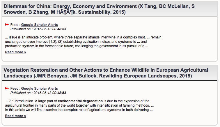
In Sux0r, here are a couple of items form the final result:

sux0rfeed

Scripts for Twitter Data

Twitter data– the endless stream of tweets, the user network, and the rise and fall of hashtags– offers a flood of insight into the minute-by-minute state of the society. Or at least one self-selecting part of it. A lot of people want to use it for research, and it turns out to be pretty easy to do so.

You can either purchase twitter data, or collect it in real-time. If you purchase twitter data, it’s all organized for you and available historically, but it basically isn’t anything that you can’t get yourself by monitoring twitter in real-time. I’ve used GNIP, where the going rate was about $500 per million tweets in 2013.

There are two main ways to collect data directly from twitter: “queries” and the “stream”. Queries let you get up to 1000 tweets at any point in time– whichever the most recent tweets that match your search criteria. The stream gives you a fraction of a percent of tweets continuously, which very quickly adds up, based on filtering criteria.

Scripts for doing these two options are below, but you need to decide on the search/streaming criteria. Typically, these are search terms and geographical constraints. See Twitter’s API documentation to decide on your search options.

Twitter uses an athentication system to identify both the individual collecting the data, and what tool is helping them do it. It is easy to register a new tool, whereby you pretend that you’re a startup with a great new app. Here are the steps:

  1. Install python’s twitter package, using “easy_install twitter” or “pip install twitter”.
  2. Create an app at http://ift.tt/1oHSTpv. Leave the callback URL blank, but fill in the rest.
  3. Set the CONSUMER_KEY and CONSUMER_SECRET in the code below to the values you get on the keys and access tokens tab of your app.
  4. Fill in the name of the application.
  5. Fill in any search terms or structured searches you like.
  6. If you’re using the downloaded scripts, which output data to a CSV file, change where the file is written, to some directory (where it says “twitter/us_”).
  7. Run the script from your computer’s terminal (i.e., python search.py)
  8. The script will pop up a browser for you to log into twitter and accept permissions from your app.
  9. Get data.

Here is what a simple script looks like:

import os, twitter

APP_NAME = "Your app name"
CONSUMER_KEY = 'Your consumer key'
CONSUMER_SECRET = 'Your consumer token'

# Do we already have a token saved?
MY_TWITTER_CREDS = os.path.expanduser('~/.class_credentials')
if not os.path.exists(MY_TWITTER_CREDS):
    # This will ask you to accept the permissions and save the token
    twitter.oauth_dance(APP_NAME, CONSUMER_KEY, CONSUMER_SECRET,
                        MY_TWITTER_CREDS)

# Read the token
oauth_token, oauth_secret = twitter.read_token_file(MY_TWITTER_CREDS)

# Open up an API object, with the OAuth token
api = twitter.Twitter(api_version="1.1", auth=twitter.OAuth(oauth_token, oauth_secret, CONSUMER_KEY, CONSUMER_SECRET))

# Perform our query
tweets = api.search.tweets(q="risky business")

# Print the results
for tweet in tweets['statuses']:
    if not 'text' in tweet:
        continue

    print tweet
    break

For automating twitter collection, I’ve put together scripts for queries (search.py), streaming (filter.py), and bash scripts that run them repeatedly (repsearch.sh and repfilter.sh). Download the scripts.

To use the repetition scripts, make the repetition scripts executable by running “chmod a+x repsearch.sh repfilter.sh“. Then run them, by typing ./repfilter.sh or ./repsearch.sh. Note that these will create many many files over time, which you’ll have to merge together.
US Water Network

The America’s Water project, coordinated at Columbia’s Water Center by Upmanu Lall, is trying to understand the US water system as an integrated whole, and understand how that system will evolve over the next decades. Doing so will require a comprehensive model, incorporating agriculture, energy, cities, policy, and more.

We are just beginning to lay the foundation for that model. A first step is to create a network of links between station gauges around the US, representing upstream and downstream flows and counties served. The ultimate form of that model will rely on physical flow data, but I created a first pass using simple rules:

  1. Every gauge can only be connected to one downstream gauge (but not visa versa).
  2. Upstream gauges must be at a higher elevation than downstream gauges.
  3. Upstream gauges must be fed by a smaller drainage basin than downstream gauges.
  4. Of the gauges that satisfy the first two constraints, the chosen downstream gauge is the one with the shortest distance and the most “plausible” streamflow.

The full description is available on Overleaf. I’ve applied the algorithm to the GAGES II database from USGSU, which includes all station gauges with at least 20 years of data.

network3

Every red dot is a gauge, black lines are upstream-downstream connections between gauges, and the blue and green lines connect counties with each of the gauges by similar rules to the ones above (green edges if the link is forced to be longer than 100 km).

This kind of network opens the door for a lot of interesting analyses. For example, if agricultural withdrawals increase in the midwest, how much less water will be available downstream? We’re working now to construct a full optimization model that accounts for upstream dependencies.

Another simple question is, how much of the demand in each county is satisfied by flows available to it? Here are the results, and many cities show up in sharp red, showing that their demands exceed the surface water by 10 times or more.

supplydemand-surface

Games from Mac Plus

About a decade ago, I got a 3.5″ floppy reader for my laptop, and every so often I’ve gone through a pile of disks seeing if anything is still readable and worth saving. I think those days are over– a metal disk protector is now stuck in the reader, and all the software available for Windows to read mac disks appears to be broken or commercial.

But my most recent pile brought back memories of many happy hours of simple and elegant games. Some day I’ll write about my latterday favorites (Armor Alley, Dark Castle, Prince of Persia) or the less-actiony BBS and World Builder games I also loved, but right now I’m remembering some space games that brought a particular joy.

Crystal Quest

Probably a precursor to Asteroids, a game made progressively more difficult by space creatures that appear first as curiosity, and eventually with furosity.

Continuum

A space game of puzzles, with a big library of widgets, and a builder of new levels.

Sitting on geodes

Sometimes I think that research is more like mining than maze-solving. Like art (I imagine), the gems that we are able to bring forth are buried inside of us. Each of us stands on a vast mineral deposit, the accumlated layers of our experiences and our unconscious foundation. By our 30’s, we’ve learned to grow a harvest in our top-soil, but we’ve also had a chance to dig deeper and get a sense of that wealth. One of the challenges of life is to ensure that we get to keep digging under our own feet.


From Saturday Morning Breakfast Cereal.

Some people pan for precious metals; others plan out whole quarries of ore. Research techniques (and philosophical modes, literary critique, drawing technique, etc.) allow us to mine at will, but each works best on certain kinds of stone. You can dig shallow, and strike oil or gas able to propell you through the economic world. You can dig deep, and get unique and precious gems, metamorphized by the heat and pressure of the unconscious mind. If you dig too deep, you hit an inpenetrable bedrock.

Me, I look for geodes. Each of these rough stones contains a cavity filled with crystals. You can tell a geode by its face, but you never know what’s inside until you break it open. I don’t like throwing away research projects, even if I don’t have time for them, because I still want to break them open. On the other hand, I know that the more I dig, the more geodes I can find. And so, I can choose to leave gems in the ground, waiting at unforetold depths.

New Years Resolutions

I love New Years resolutions. A ritual opportunity to adjust the choices that make up life. Like everyone, I struggle (read: give up frequently) on them, but part of the joy is to understand that process and resolve better.

I’m expecting a big semester, starting soon: my Complexity Science course, bigger and better; finishing my thesis; being substantively involved in three large projects and several small ones; and getting a job. My theory of organization this time is to schedule– my work days are specified to the hour on the projects I hope to finish by the end of the semester:
schedule

My resolutions are mostly following the same idea, recognizing time less as a limiting factor than as an organizing principle:

  • Additional morning exercise (15 min. / week)
  • Personal or professional blogging (30 min. / week)
  • Review my colleagues interests and activities (30 min. / week) [next year follow-up: usefully encode my network]
  • Write to distant friends (30 min. / week)
  • Deep reflection on goals and activities (1 hr. / week)
  • Go for a hike outside the city in every month [next year follow-up: hike the same trail every month of the year]
  • Read a journal cover-to-cover every week [next year follow-up: become a regular reader of one journal]

Negative result: country-wide growing degree-days

I put this here as a warning. While growing degree-days (GDD) are well-known as an effective model to predict yields, they don’t perform so hot at the country-scale.

I used mean temperature GDDs, between 8 and 24 degrees C, estimated at many locations from station data, and then using the weighted average by production within each country. Here are the results:

Statistical models
Barley Maize Millet Rice Sorghum Wheat
GDD / 1000 -0.03 0.01 -0.07** 0.08 0.04* -0.08***
(0.01) (0.01) (0.03) (0.06) (0.02) (0.02)
Precip. (m) 0.09 0.11*** 0.12* 0.02 0.14*** -0.04
(0.05) (0.03) (0.05) (0.03) (0.04) (0.04)
Country Cubic Y Y Y Y Y Y
R2 0.95 0.97 0.91 0.97 0.92 0.96
Adj. R2 0.94 0.96 0.90 0.97 0.91 0.95
Num. obs. 1639 3595 1516 1721 2300 1791
***p < 0.001, **p < 0.01, *p < 0.05

As you can see, for most crops, these GDDs aren’t even significant, and as frequently negative as positive. This defies a century of agricultural research, but the same data at a fine spatial scale seems to work just fine.

Growing Degree-Day Calculations

Schlenker and Roberts (2009) use daily minimum and maximum temperatures to calculate growing degrees, rather than daily mean temperatures. This is important when the effect of extreme temperatures is an issue, since these often will not show up in mean temperatures.

Growing degree days form a useful model of crop productivity. DMAS has examples of these for maize, soybeans, and cotton.

To do this, they use a sinusoidal approximation, integrating the area of a curve through the minimum and maximum temperatures:
thresholds
(adapted from here– but don’t use their calculations!)

The calculations aren’t very difficult, but require some careful math. I had a need to write them in python and translate them to R, so I’m providing them here for anyone’s benefit.

import numpy as np
import warnings

warnings.simplefilter("ignore", RuntimeWarning)

def above_threshold(mins, maxs, threshold):
    """Use a sinusoidal approximation to estimate the number of Growing
Degree-Days above a given threshold, using daily minimum and maximum
temperatures.

mins and maxs are numpy arrays; threshold is in the same units."""

    # Determine crossing points, as a fraction of the day
    plus_over_2 = (mins + maxs)/2
    minus_over_2 = (maxs - mins)/2
    two_pi = 2*np.pi
    # d0s is the times of crossing above; d1s is when cross below
    d0s = np.arcsin((threshold - plus_over_2) / minus_over_2) / two_pi
    d1s = .5 - d0s

    # If always above or below threshold, set crossings accordingly
    aboves = mins >= threshold
    belows = maxs <= threshold

    d0s[aboves] = 0
    d1s[aboves] = 1
    d0s[belows] = 0
    d1s[belows] = 0

    # Calculate integral
    F1s = -minus_over_2 * np.cos(2*np.pi*d1s) / two_pi + plus_over_2 * d1s
    F0s = -minus_over_2 * np.cos(2*np.pi*d0s) / two_pi + plus_over_2 * d0s
    return np.sum(F1s - F0s - threshold * (d1s - d0s))

def get_gddkdd(mins, maxs, gdd_start, kdd_start):
    """Get the Growing Degree-Days, as degree-days between gdd_start and
kdd_start, and Killing Degree-Days, as the degree-days above
kdd_start.

mins and maxs are numpy arrays; threshold is in the same units."""

    dd_lowup = above_threshold(mins, maxs, gdd_start)
    dd_above = above_threshold(mins, maxs, kdd_start)
    dd_lower = dd_lowup - dd_above

    return (dd_lower, dd_above)

Download the code for R or python.

Sustainability, Engineering, and Philosophy